Bayesian quadrature weighting example

The aim of this page is to provide a simple example to compute optimal-weights for quadrature on any given sample.

import numpy as np
import openturns as ot
import otkerneldesign as otkd
import matplotlib.pyplot as plt
from matplotlib import cm

The following helper class will make plotting easier.

class DrawFunctions:
    def __init__(self):
        dim = 2
        self.grid_size = 100
        lowerbound = [0.] * dim
        upperbound = [1.] * dim
        mesher = ot.IntervalMesher([self.grid_size-1] * dim)
        interval = ot.Interval(lowerbound, upperbound)
        mesh = mesher.build(interval)
        self.nodes = mesh.getVertices()
        self.X0, self.X1 = np.array(self.nodes).T.reshape(2, self.grid_size, self.grid_size)

    def draw_2D_contour(self, title, function=None, distribution=None, colorbar=cm.coolwarm):
        fig = plt.figure(figsize=(7, 6))
        if distribution is not None:
            Zpdf = np.array(distribution.computePDF(self.nodes)).reshape(self.grid_size, self.grid_size)
            nb_isocurves = 9
            contours = plt.contour(self.X0, self.X1, Zpdf, nb_isocurves, colors='black', alpha=0.6)
            plt.clabel(contours, inline=True, fontsize=8)
        if function is not None:
            Z = np.array(function(self.nodes)).reshape(self.grid_size, self.grid_size)
            plt.contourf(self.X0, self.X1, Z, 18, cmap=colorbar)
            plt.colorbar()
        plt.title(title)
        plt.xlabel("$x_0$")
        plt.ylabel("$x_1$")
        return fig

    def draw_candidates(self, candidate_sample, title='Design of experiments'):
        fig = d.draw_2D_contour(title, None, distribution)
        plt.title(title)
        plt.xlabel("$x_0$")
        plt.ylabel("$x_1$")
        plt.scatter(candidate_sample[:, 0], candidate_sample[:, 1], alpha=0.1, label='candidate points ($N={}$)'.format(len(candidate_sample)), color='C7')
        plt.legend(loc='best')
        return fig

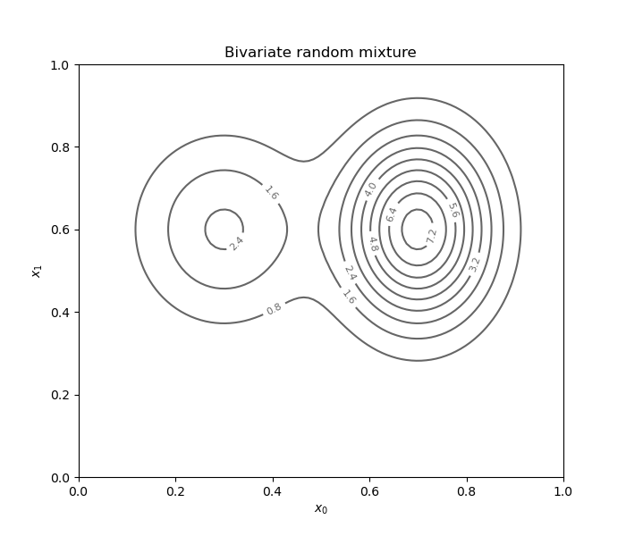
Dependent bivariate random mixture

Let us first define an independent bivariate random mixture.

modes = [ot.Normal(0.3, 0.12), ot.Normal(0.7, 0.1)]
weight = [0.4, 1.0]
mixture = ot.Mixture(modes, weight)
normal = ot.Normal(0.6, 0.15)
distribution = ot.ComposedDistribution([mixture, normal])

Draw a contour plot of the PDF.

d = DrawFunctions()
fig = d.draw_2D_contour('Bivariate random mixture', None, distribution)
plt.show()

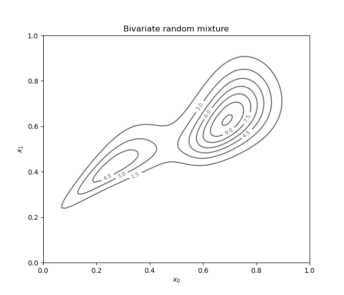
Using the same example, we can add a Copula as a dependency structure. Note that the KernelHerdingTensorized class cannot be used in this case.

distribution.setCopula(ot.ClaytonCopula(2.))
fig = d.draw_2D_contour('Bivariate random mixture', None, distribution)
plt.show()

Define a kernel.

dimension = distribution.getDimension()
ker_list = [ot.MaternModel([0.1], [1.0], 2.5)] * dimension
kernel = ot.ProductCovarianceModel(ker_list)

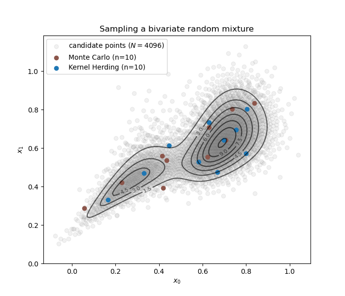
We build both Monte Carlo and kernel herding designs representative of the distribution.

size = 10
mc_design = distribution.getSample(size)
kh = otkd.KernelHerding(
    kernel=kernel,
    candidate_set_size=2 ** 12,
    distribution=distribution
)
kh_design = kh.select_design(size)

Draw the designs and the empirical representation of the target distribution (a.k.a., candidate set).

fig = d.draw_candidates(kh._candidate_set, 'Sampling a bivariate random mixture')
plt.scatter(mc_design[:, 0], mc_design[:, 1], label='Monte Carlo (n={})'.format(size), marker='o', color='C5')
plt.scatter(kh_design[:, 0], kh_design[:, 1], label='Kernel Herding (n={})'.format(size), marker='o', color='C0')
plt.legend(loc='best')
#plt.legend(bbox_to_anchor=(0.5, -0.1), loc='upper center') # outside bounds
plt.show()

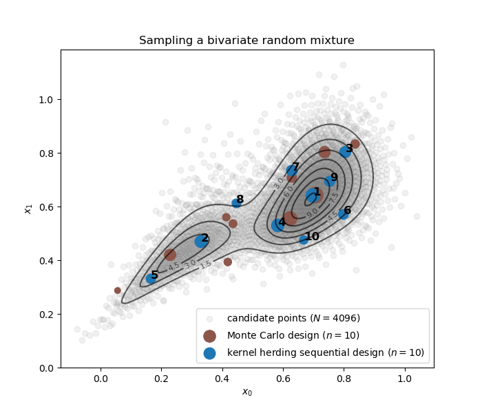
Bayesian quadrature weights

For any given sample and target distribution, let us compute a set of optimal weights for quadrature.

bqm = otkd.BayesianQuadratureWeighting(
    kernel=kernel,
    distribution=distribution,
)
kh_weights = bqm.compute_bayesian_quadrature_weights(kh_design)
mc_weights = bqm.compute_bayesian_quadrature_weights(mc_design)

Draw samples with corresponding weights proportionate to the markers sizes.

fig = d.draw_candidates(kh._candidate_set, 'Sampling a bivariate random mixture')
x_label = '{} sequential design ($n={}$)'.format('kernel herding', len(kh_design))
plt.scatter(mc_design[:, 0], mc_design[:, 1], color='C5', label='Monte Carlo design ($n={}$)'.format(len(mc_design)), s=mc_weights * 1500, marker='o')
plt.scatter(kh_design[:, 0], kh_design[:, 1], color='C0', label=x_label, s=kh_weights * 1500, marker='o')
for i in range(len(kh_design)):
    plt.text(kh_design[i][0], kh_design[i][1], "{}".format(i + 1), weight="bold", fontsize=12)
plt.legend(loc='best')
plt.show()