Machine learning validation example

The aim of this page is to provide simple use-case where kernel design is used to build a design of experiments complementary to an existing one, either to enhance a machine learning model or for validation.

import numpy as np
import openturns as ot
import otkerneldesign as otkd
import matplotlib.pyplot as plt
from matplotlib import cm

The following helper class will make plotting easier.

class DrawFunctions:
    def __init__(self):
        dim = 2
        self.grid_size = 100
        lowerbound = [0.] * dim
        upperbound = [1.] * dim
        mesher = ot.IntervalMesher([self.grid_size-1] * dim)
        interval = ot.Interval(lowerbound, upperbound)
        mesh = mesher.build(interval)
        self.nodes = mesh.getVertices()
        self.X0, self.X1 = np.array(self.nodes).T.reshape(2, self.grid_size, self.grid_size)

    def draw_2D_contour(self, title, function=None, distribution=None, colorbar=cm.viridis):
        fig = plt.figure(figsize=(7, 6))
        if distribution is not None:
            Zpdf = np.array(distribution.computePDF(self.nodes)).reshape(self.grid_size, self.grid_size)
            nb_isocurves = 9
            contours = plt.contour(self.X0, self.X1, Zpdf, nb_isocurves, colors='black', alpha=0.6)
            plt.clabel(contours, inline=True, fontsize=8)
        if function is not None:
            Z = np.array(function(self.nodes)).reshape(self.grid_size, self.grid_size)
            plt.contourf(self.X0, self.X1, Z, 18, cmap=colorbar)
            plt.colorbar()
        plt.title(title)
        plt.xlabel("$x_0$")
        plt.ylabel("$x_1$")
        return fig

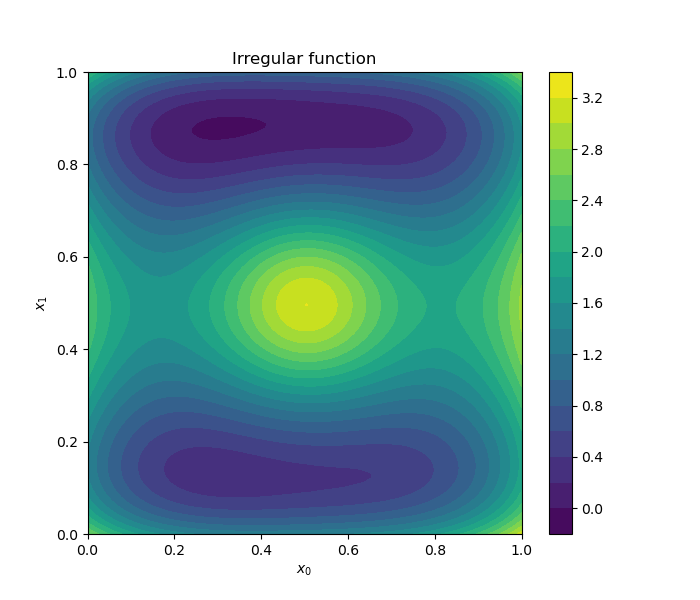
Regression model of a 2D function

Define the function to be approximated.

function_expression = 'exp((2*x1-1))/5 - (2*x2-1)/5 + ((2*x2-1)^6)/3 + 4*((2*x2-1)^4) - 4*((2*x2-1)^2) + (7/10)*((2*x1-1)^2) + (2*x1-1)^4 + 3/(4*((2*x1-1)^2) + 4*((2*x2-1)^2) + 1)'
irregular_function = ot.SymbolicFunction(['x1', 'x2'], [function_expression])
irregular_function.setName("Irregular")
print(irregular_function)

[x1,x2]->[exp((2*x1-1))/5 - (2*x2-1)/5 + ((2*x2-1)^6)/3 + 4*((2*x2-1)^4) - 4*((2*x2-1)^2) + (7/10)*((2*x1-1)^2) + (2*x1-1)^4 + 3/(4*((2*x1-1)^2) + 4*((2*x2-1)^2) + 1)]

Draw a contours of the 2D function.

d = DrawFunctions()
d.draw_2D_contour("Irregular function", function=irregular_function)
plt.show()

Define the joint input random vector, here uniform since our goal is to build a good regression model on the entire domain.

distribution = ot.ComposedDistribution([ot.Uniform(0, 1)] * 2)

Build a learning set, for example by Latin Hypercube Sampling.

learning_size = 20
ot.RandomGenerator.SetSeed(0)
LHS_experiment = ot.LHSExperiment(distribution, learning_size, True, True)
x_learn = LHS_experiment.generate()
y_learn = irregular_function(x_learn)

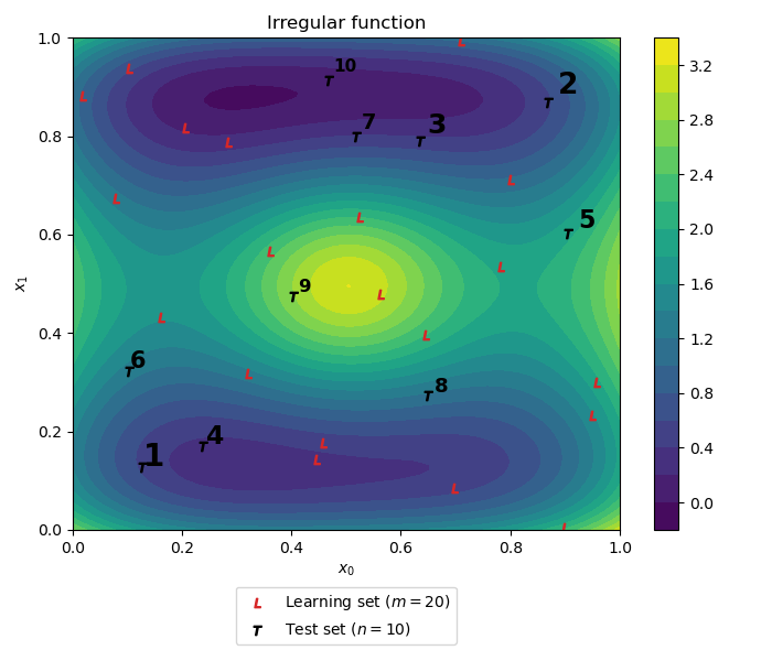
Build a design of experiments complementary to the existing learning set (e.g., for testing). Note that the kernel herding method could also be used.

test_size = 10
sp = otkd.GreedySupportPoints(distribution, initial_design=x_learn)
x_test = sp.select_design(test_size)
y_test = irregular_function(x_test)

Plot the Learning set (in red) and testing sets (in black with the corresponding construction design order).

fig = d.draw_2D_contour("Irregular function", function=irregular_function)
plt.scatter(x_learn[:, 0], x_learn[:, 1], label='Learning set ($m={}$)'.format(len(x_learn)), marker='$L$', color='C3')
plt.scatter(x_test[:, 0], x_test[:, 1], label='Test set ($n={}$)'.format(len(x_test)), marker='$T$', color='k')
# Test set indexes
[plt.text(x_test[i][0] * 1.02, x_test[i][1] * 1.02, str(i + 1), weight="bold", fontsize=np.max((20 - i, 5))) for i in range(test_size)]
lgd = plt.legend(bbox_to_anchor=(0.5, -0.1), loc='upper center')
plt.tight_layout(pad=1)
plt.show()

Kriging model fit and validation

Build a simple Kriging regression model.

dim = distribution.getDimension()
basis = ot.ConstantBasisFactory(dim).build()
covariance_model = ot.MaternModel([0.2] * dim, 2.5)
algo = ot.KrigingAlgorithm(x_learn, y_learn, covariance_model, basis)
algo.run()
result = algo.getResult()
kriging_model = result.getMetaModel()

Build a large Monte Carlo reference test set and compute a reference performance metric on it.

xref_test = distribution.getSample(10000)
yref_test = irregular_function(xref_test)
ref_val = ot.MetaModelValidation(xref_test, yref_test, kriging_model)
ref_Q2 = ref_val.computePredictivityFactor()[0]
print("Reference Monte Carlo (n=10000) predictivity coefficient: {:.3}".format(ref_Q2))

Reference Monte Carlo (n=10000) predictivity coefficient: 0.828

In comparison, our test set underestimates the performance of the Kriging model. This situation is expected since the test points are supposed to be far from the learning set.

val = ot.MetaModelValidation(x_test, y_test, kriging_model)
estimated_Q2 = val.computePredictivityFactor()[0]
print("Support points (n={}) predictivity coefficient: {:.3}".format(test_size, estimated_Q2))

Support points (n=10) predictivity coefficient: 0.758

To take this into account, let us compute optimal weights for validation. After applying the weights, the estimated performance is more optimistic and closer to the reference value.

tsw = otkd.TestSetWeighting(x_learn, x_test, sp._candidate_set)
optimal_test_weights = tsw.compute_weights()
weighted_Q2 = 1 - np.mean(np.array(y_test).flatten() * optimal_test_weights) / y_test.computeVariance()[0]
print("Weighted support points (n={}) predictivity coefficient: {:.3}".format(test_size, weighted_Q2))

Weighted support points (n=10) predictivity coefficient: 0.871

Adding test set to learning set

The test set can now be added to the learning set to enhance the Kriging model

x_learn.add(x_test)
y_learn.add(y_test)
algo_enhanced = ot.KrigingAlgorithm(x_learn, y_learn, covariance_model, basis)
algo_enhanced.run()
result_enhanced = algo_enhanced.getResult()
kriging_enhanced = result_enhanced.getMetaModel()

ref_val_enhanced = ot.MetaModelValidation(xref_test, yref_test, kriging_enhanced)
ref_Q2_enhanced = ref_val_enhanced.computePredictivityFactor()[0]
print("Enhanced Kriging - Monte Carlo (n=10000) predictivity coefficient: {:.3}".format(ref_Q2_enhanced))

Enhanced Kriging - Monte Carlo (n=10000) predictivity coefficient: 0.922