Kernel herding examples

The aim of this page is to provide simple examples where kernel herding is applied to multivariate random inputs with or without a dependency structure.

import numpy as np
import openturns as ot
import otkerneldesign as otkd
import matplotlib.pyplot as plt
from matplotlib import cm

The following helper class will make plotting easier.

class DrawFunctions:
    def __init__(self):
        dim = 2
        self.grid_size = 100
        lowerbound = [0.] * dim
        upperbound = [1.] * dim
        mesher = ot.IntervalMesher([self.grid_size-1] * dim)
        interval = ot.Interval(lowerbound, upperbound)
        mesh = mesher.build(interval)
        self.nodes = mesh.getVertices()
        self.X0, self.X1 = np.array(self.nodes).T.reshape(2, self.grid_size, self.grid_size)

    def draw_2D_contour(self, title, function=None, distribution=None, colorbar=cm.coolwarm):
        fig = plt.figure(figsize=(7, 6))
        if distribution is not None:
            Zpdf = np.array(distribution.computePDF(self.nodes)).reshape(self.grid_size, self.grid_size)
            nb_isocurves = 9
            contours = plt.contour(self.X0, self.X1, Zpdf, nb_isocurves, colors='black', alpha=0.6)
            plt.clabel(contours, inline=True, fontsize=8)
        if function is not None:
            Z = np.array(function(self.nodes)).reshape(self.grid_size, self.grid_size)
            plt.contourf(self.X0, self.X1, Z, 18, cmap=colorbar)
            plt.colorbar()
        plt.title(title)
        plt.xlabel("$x_0$")
        plt.ylabel("$x_1$")
        return fig

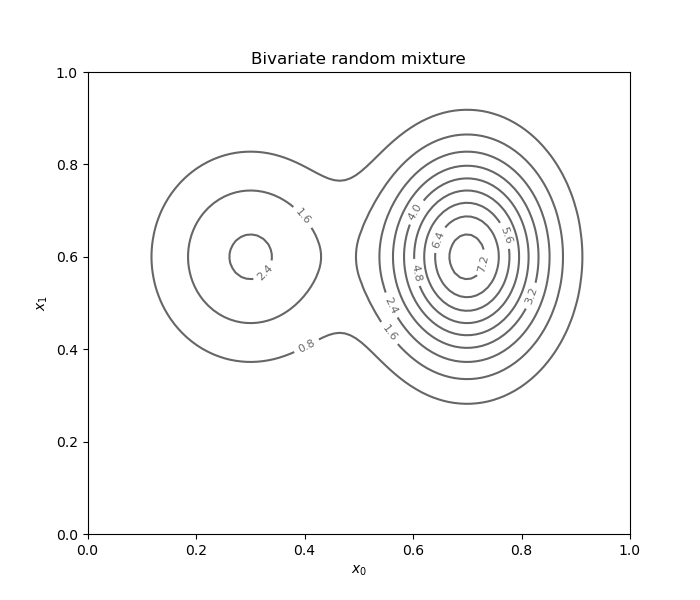
Independent bivariate random mixture

modes = [ot.Normal(0.3, 0.12), ot.Normal(0.7, 0.1)]
weight = [0.4, 1.0]
mixture = ot.Mixture(modes, weight)
normal = ot.Normal(0.6, 0.15)
distribution = ot.ComposedDistribution([mixture, normal])

Draw a contour plot of the PDF.

d = DrawFunctions()
fig = d.draw_2D_contour('Bivariate random mixture', None, distribution)
plt.show()

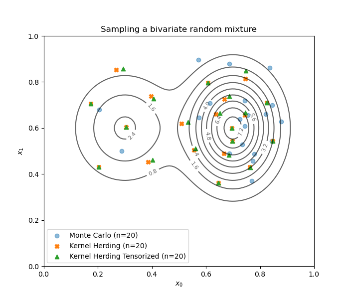
First, sample from the distribution to get a Monte-Carlo design.

dimension = distribution.getDimension()
size = 20
mc_design = distribution.getSample(size)

Define a kernel.

ker_list = [ot.MaternModel([0.1], [1.0], 2.5)] * dimension
kernel = ot.ProductCovarianceModel(ker_list)

Build a kernel herding-based design representative of the distribution.

kh = otkd.KernelHerding(
    kernel=kernel,
    candidate_set_size=2 ** 12,
    distribution=distribution
)
kh_design = kh.select_design(size)

Because the copula of the distribution is independent and we used a product kernel, the KernelHerdingTensorized class can do this in a computationally more efficient way.

kht = otkd.KernelHerdingTensorized(
    kernel=kernel,
    candidate_set_size=2 ** 12,
    distribution=distribution
)
kht_design = kht.select_design(size)

Draw the designs.

fig = d.draw_2D_contour('Sampling a bivariate random mixture', None, distribution)
plt.scatter(mc_design[:, 0], mc_design[:, 1], label='Monte Carlo (n={})'.format(size), marker='o', alpha=0.5)
plt.scatter(kh_design[:, 0], kh_design[:, 1], label='Kernel Herding (n={})'.format(size), marker='X', color='C1')
plt.scatter(kht_design[:, 0], kht_design[:, 1], label='Kernel Herding Tensorized (n={})'.format(size), marker='^', color='C2')
plt.legend()
#plt.legend(bbox_to_anchor=(0.5, -0.1), loc='upper center') # outside bounds
plt.show()

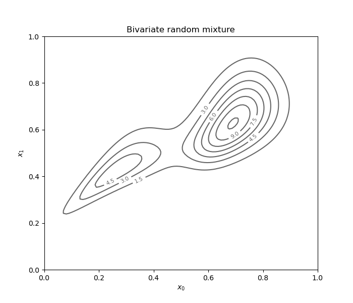
Dependent bivariate random mixture

Using the same example, we can add a Copula as a dependency structure. Note that the KernelHerdingTensorized class cannot be used in this case.

distribution.setCopula(ot.ClaytonCopula(2.))
fig = d.draw_2D_contour('Bivariate random mixture', None, distribution)
plt.show()

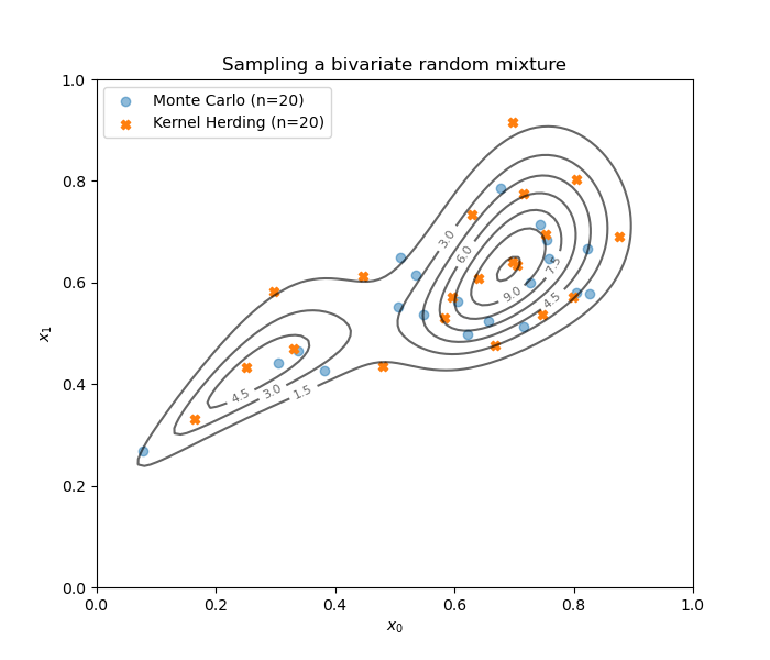
We build both Monte Carlo and kernel herding designs.

mc_design = distribution.getSample(size)
kh = otkd.KernelHerding(
    kernel=kernel,
    candidate_set_size=2 ** 12,
    distribution=distribution
)
kh_design = kh.select_design(size)

Draw the designs.

fig = d.draw_2D_contour('Sampling a bivariate random mixture', None, distribution)
plt.scatter(mc_design[:, 0], mc_design[:, 1], label='Monte Carlo (n={})'.format(size), marker='o', alpha=0.5)
plt.scatter(kh_design[:, 0], kh_design[:, 1], label='Kernel Herding (n={})'.format(size), marker='X', color='C1')
plt.legend()
#plt.legend(bbox_to_anchor=(0.5, -0.1), loc='upper center') # outside bounds
plt.show()